Quantifying Expression in Single Cell

Measuring gene expression levels within individual cells.

Author

Affiliation

Wajid Iqbal

International Islamic University, Islamabad

Part2:

Disclaimer: ⚠️ This post may be lengthy for some readers, so please adjust accordingly. Welcome to the second blog in our series on single-cell RNA sequencing (scRNA-seq). In this blog, we will discuss various transcript quantification methods and some of the problems associated with quantification. Most of the content discussed here relates to the droplet-based method of scRNA-seq.

Transcript Quantification:

Transcript quantification is the process of measuring the abundance of RNA transcripts (messenger RNA or mRNA) within a sample. In the context of single-cell RNA sequencing (scRNA-seq), it involves determining the number of RNA molecules corresponding to each gene in individual cells.The general workflow for single cell library construction is shown in Figure 1

Figure 1: General Workflow for single cell Library Construction.

There are two major version of Transcript Quantification: Full-length and tag-based.

Full length:

• This method makes an attempt to cover the whole transcript with sequencing reads.

Based on the type of methods used for transcript quantification, can have a serious impact on the number of genes captured, so try to asses all the available methods and use the approach that best suits your study.

• Only plate-based protocols can perform Full-length sequencing.

• Full-length protocols do not always ensure even coverage of transcripts, leading to potential biases in specific regions across the gene body.

• The only advantage that full length based approach provides, is the detection of splice site variants.

Tag-based Protocols:

Tag-based protocols sequence only the 3’ or 5’ ends of transcripts, which limits full gene coverage and complicates the alignment of reads to specific transcripts and the differentiation of isoforms. However, these protocols enable the use of unique molecular identifiers (UMIs), which help correct biases in transcript amplification. Although this is beyond the scope of this blog to discuss in detail each approach and platform used for sc-RNASeq but down below is a summarized table that contains all the information related to the platform name and separation methods used in each approach.

library(gt)
scRNA_seq_data <- data.frame(
  Platform_Name = c("VASA-seq", "Smart-seq3", "DNBelabC4", "Seq-Well", "MATQ-seq", "10× Genomics", "Cyto-Seq", "SC3-seq", "inDrop-seq", "Drop-seq", "MARS-seq", "STRT-seq", "Quartz-seq", "Fluidigm C1", "Smart-seq2", "Smart-seq", "CEL-seq", "Tang-2009"),
  Separation_Method = c("FANS", "Microfluidics", "Microfluidics", "Microfluidics", "FACS", "Microfluidics", "Microfluidics", "Micromanipulation", "Microfluidics", "Microfluidics", "FACS", "Microfluidics", "FACS", "Microfluidics", "FACS", "FACS", "FACS", "FACS"),
  Amplification_Method = c("PCR", "PCR", "PCR", "PCR", "PCR", "PCR", "PCR", "PCR", "IVT", "PCR", "IVT", "PCR", "PCR", "PCR", "PCR", "PCR", "IVT", "PCR"),
  Using_UMI = c("YES", "YES", "YES", "YES", "YES", "YES", "YES", "YES", "YES", "YES", "YES", "NO", "YES", "NO", "NO", "NO", "YES", "NO"),
  Amplification_Range = c("All transcripts", "5′ end", "All transcripts", "3′ end", "All transcripts", "3′ end", "3′ end", "3′ end", "3′ end", "3′ end", "3′ end", "All transcripts", "3′ end", "All transcripts", "All transcripts", "All transcripts", "3′ end", "3′ end"),
  Advantages = c("Low cost and accurate dosing", "High sensitivity", "Precise quantification", "Low cost and precise quantification", "Precise quantification", "High cell capture efficiency, fast cycle time, high cell suitability, and reproducibility", "Low cost and high throughput", "Good reproducibility and accurate quantification", "Low cost and linear amplification", "Low cost and high throughput", "High specificity", "Accurate positioning of transcripts at the 5′ end to reduce amplification bias", "High sensitivity, reproducibility, and operational simplicity", "Simple process", "Full-length cDNA detects structural and RNA shear variants", "High sensitivity to reduce the rates of nucleic acid loss", "Good reproducibility and highly sensitive", "Good reproducibility"),
  Disadvantages = c("/", "Time-consuming", "/", "Unsuitable for variable splicing and allelic expression", "Low cell throughput", "Sequencing can be performed only for the 3′ end", "Cross-contamination between RNAs", "Recognize DNA at the 3′ end", "Long operating time and high initial cell concentration", "Low cell capture rate", "Low amplification efficiency", "Low sensitivity, only available for identification of 5′ end DNA", "Higher noise levels", "High cost and low throughput", "High cost, low throughput, and time-consuming", "Low throughput and the existence of transcript length bias", "Low throughput and amplification efficiency, library biased toward the 3′ end of the gene", "High cost and low throughput"),
  Release_Date = c("2022", "2020", "2019", "2017", "2017", "2016", "2015", "2015", "2015", "2015", "2014", "2014", "2013", "2013", "2013", "2012", "2012", "2009")
)

scRNA_seq_table <- gt(scRNA_seq_data) %>%
  tab_header(
    title = md("**Comparison of Different ScRNA-Seq Technology Approaches**")
  ) %>%
  cols_label(
    Platform_Name = "Platform Name",
    Separation_Method = "Separation Method",
    Amplification_Method = "Amplification Method",
    Using_UMI = "Using UMI",
    Amplification_Range = "Amplification Range",
    Advantages = "Advantages",
    Disadvantages = "Disadvantages",
    Release_Date = "Release Date"
  ) %>%
 tab_style(
    style = list(
      cell_text(weight = "bold")
    ),
    locations = cells_column_labels(everything())
  ) %>% 
  tab_source_note(source_note = md("**Reference**: Shou wang et al., The Evolution of Single-Cell RNA Sequencing Technology and Application: Progress and Perspectives.")) %>% 
  opt_stylize(style = 6, color ='gray') %>% 
  tab_options(heading.align = 'center',
              heading.background.color = 'darkgreen',
              heading.title.font.size = px(20))
scRNA_seq_table |> as_raw_html()

Comparison of Different ScRNA-Seq Technology Approaches
Platform Name	Separation Method	Amplification Method	Using UMI	Amplification Range	Advantages	Disadvantages	Release Date
VASA-seq	FANS	PCR	YES	All transcripts	Low cost and accurate dosing	/	2022
Smart-seq3	Microfluidics	PCR	YES	5′ end	High sensitivity	Time-consuming	2020
DNBelabC4	Microfluidics	PCR	YES	All transcripts	Precise quantification	/	2019
Seq-Well	Microfluidics	PCR	YES	3′ end	Low cost and precise quantification	Unsuitable for variable splicing and allelic expression	2017
MATQ-seq	FACS	PCR	YES	All transcripts	Precise quantification	Low cell throughput	2017
10× Genomics	Microfluidics	PCR	YES	3′ end	High cell capture efficiency, fast cycle time, high cell suitability, and reproducibility	Sequencing can be performed only for the 3′ end	2016
Cyto-Seq	Microfluidics	PCR	YES	3′ end	Low cost and high throughput	Cross-contamination between RNAs	2015
SC3-seq	Micromanipulation	PCR	YES	3′ end	Good reproducibility and accurate quantification	Recognize DNA at the 3′ end	2015
inDrop-seq	Microfluidics	IVT	YES	3′ end	Low cost and linear amplification	Long operating time and high initial cell concentration	2015
Drop-seq	Microfluidics	PCR	YES	3′ end	Low cost and high throughput	Low cell capture rate	2015
MARS-seq	FACS	IVT	YES	3′ end	High specificity	Low amplification efficiency	2014
STRT-seq	Microfluidics	PCR	NO	All transcripts	Accurate positioning of transcripts at the 5′ end to reduce amplification bias	Low sensitivity, only available for identification of 5′ end DNA	2014
Quartz-seq	FACS	PCR	YES	3′ end	High sensitivity, reproducibility, and operational simplicity	Higher noise levels	2013
Fluidigm C1	Microfluidics	PCR	NO	All transcripts	Simple process	High cost and low throughput	2013
Smart-seq2	FACS	PCR	NO	All transcripts	Full-length cDNA detects structural and RNA shear variants	High cost, low throughput, and time-consuming	2013
Smart-seq	FACS	PCR	NO	All transcripts	High sensitivity to reduce the rates of nucleic acid loss	Low throughput and the existence of transcript length bias	2012
CEL-seq	FACS	IVT	YES	3′ end	Good reproducibility and highly sensitive	Low throughput and amplification efficiency, library biased toward the 3′ end of the gene	2012
Tang-2009	FACS	PCR	NO	3′ end	Good reproducibility	High cost and low throughput	2009
Reference: Shou wang et al., The Evolution of Single-Cell RNA Sequencing Technology and Application: Progress and Perspectives.

• Since Tag-based methods involves sequencing only specific parts of each RNA molecule such as 3’ or 5’ ends, this allows for the efficient capture and sequencing of RNA from a large number of cell, allowing better identity of cell type population.

• Tag-based methods have usually cheaper per cell cost.

Figure 2: Whole picture of how the reads are synthesized

To capture the mRNA molecule, we hybridize it to a poly-dT sequence that has unique molecular identifier (UMI) attached to it. UMIs are randomly synthesized sequences, typically between 8 and 12 base pairs in length, depending on the technology and its version, providing over 50,000 possible combinations(Archer et al. 2016).

Possible combination with 8 and 12 bp:

Since there are 4 nucleotides (A, T, C, G)

For a UMI of 8 base pairs, there are 4^8 (65,536) possible combinations. For 12 base pairs, the number of combinations is 4^12(16,777,216).

Theoretically, each mRNA molecule would have a unique barcode. However, in practice, randomness in synthesis does not guarantee equal probability for all sequences, leading to biases in UMI distribution. To address this, we combine the UMI with the genomic location of the mRNA transcript to uniquely identify captured mRNA molecules.

Additionally, we incorporate a cell barcode, a sequence between 14 and 18 base pairs, the number varies with the technology used. These barcodes are deliberately generated from predetermined pools, ensuring each barcode differs by at least two base pairs from any other to allow for error correction.

More explanation on barcodes:

When we design barcodes to identify each cell, we make sure every barcode is different from every other barcode by at least two letters. This way, even if there’s a small mistake in reading the barcode (like reading an ‘A’ as a ‘T’), we can still tell which cell it’s supposed to be from. If two barcodes are only one letter different, we assume the difference is just a mistake and group them together as coming from the same cell. This helps us correct for small errors and ensures we correctly identify each cell.

Sequencing errors can occur, and having such errors in cell barcodes could misassign reads to incorrect cell types, such as assigning a read from a T-cell to an endothelial cell. The two base pair differences between barcodes enable us to aggregate barcodes with single base pair differences, treating them as sequencing errors, and ensuring they all originated from the same cell (Aird et al. 2011).

More on UMI and barcodes

UMIs are used to identify and quantify individual RNA molecules within a single cell. They help correct for biases introduced during the amplification process (such as PCR) by allowing the differentiation between true biological duplicates and duplicates introduced during amplification. When an RNA molecule is captured and converted to cDNA, a unique sequence (UMI) is attached to it. This UMI allows researchers to count the original number of RNA molecules more accurately because even if the molecule is amplified multiple times, it will still have the same UMI.

While cell barcodes are used to identify which cell an RNA molecule came from and essential for distinguish RNA molecule from different cells. Each cell in the experiment is tagged with a unique barcode before sequencing and then this barcode is added to all the RNA molecules captured from that particular cell.

Knowing the predetermined pool of barcode sequences is essential for accurate identification and error correction in our analysis.We need to be aware of the specific pool of barcodes used. For example, if you are using the 10X Genomics Chromium system, 10X genomics barcode whitelist you can visit their website to identify the version you are using and download the corresponding whitelist of barcodes.Below shown in Figure 3 is whitelist corresponding to different chemistry of 10X Genomics with its bp as well.

Figure 3: Whitelist of the barcodes for 10X chromium system

If you are using a different technology, you will need to locate the appropriate whitelist of barcodes for that system.

Note

Note that barcode lengths and sequences can vary between versions, so it is crucial to ensure you have the correct one. the good thing is that cell-Ranger pipeline has most of these built in and will automatically try and guess which white list you’re using but it’s always preferable to know ahead of time and tell it the right one so that you have 0% chance of it guessing the wrong one.

After barcodes, the next step is PCR Amplification, We then obtain our PCR primers, which are use to extensively amplify our mRNA molecules, increasing their quantity from picograms to nanograms or more for our sequencing libraries. Once hybridized, a reverse transcriptase primer is also attached, enabling reverse transcription to begin and generate a cDNA strand from the mRNA. This process includes adding a series of cytosines (C’s) at the end of the cDNA. A switch oligo is then added, which hybridizes to these poly-C tails and provides a primer for reverse transcriptase to synthesize the second strand of cDNA as shown in Figure 2.

Afterward, we have our cDNA with PCR primers, which we can amplify. We perform the amplification through 12 to 15 PCR cycles. Any inefficiencies or noise in the PCR process are also amplified, which is why we use unique molecular identifiers (UMIs). UMIs help eliminate amplification noise by counting the unique UMIs instead of the total reads at the end.

Next, sequencing library is prepared. For Illumina sequencing, this involves fragmenting the cDNA into approximately 300 base pair fragments, followed by paired-end sequencing to generate two 100 base pair reads. Some sequencing facilities now offer protocols specifically optimized for 10X Genomics data, sequencing only the required lengths for each read. so in totality this is how scrna single read looks like shown in Figure 4 :

Figure 4: Image credit Tallulah Andrews Presentation, Andrews Computational Biology Lab: Structure of scRNA-seq reads

Based on the above discussion, lets ask some question and then try to answer those.

Q1: What would happen if the mRNA gets highly degraded before reverse transcription occurs?

Ans1: if the mRNA is degraded then their are several possible scenarios that works in connection with each other can be disrupted:

• Fragmented mRNA may not include the entire sequence of the genes. This can lead to missing information for genes that are represented only by the degraded parts.

• The sequencing library may become biased towards the more stable fragments of mRNA, potentially overrepresenting some parts of the transcriptome while underrepresenting others. This can skew the expression profiles.

• Incomplete cDNA Synthesis.

Q2: What would happen if the wrong cell barcode whitelist is used ?

Ans2: This would cause alot of the reads to not match to any cell essentially resulting in throwing away 70 or 80% of reads because cell Ranger will not be able to map them to a cell.

Q3: what would happen if their is a strong bias towards certain sequences when generating UMIs.

Ans3: The strong bias towards certains sequences would undercount the amount of mRNA molecules actually captured because we will get more mRNA molecules with the same UMI.

Raw data to count-matrix:

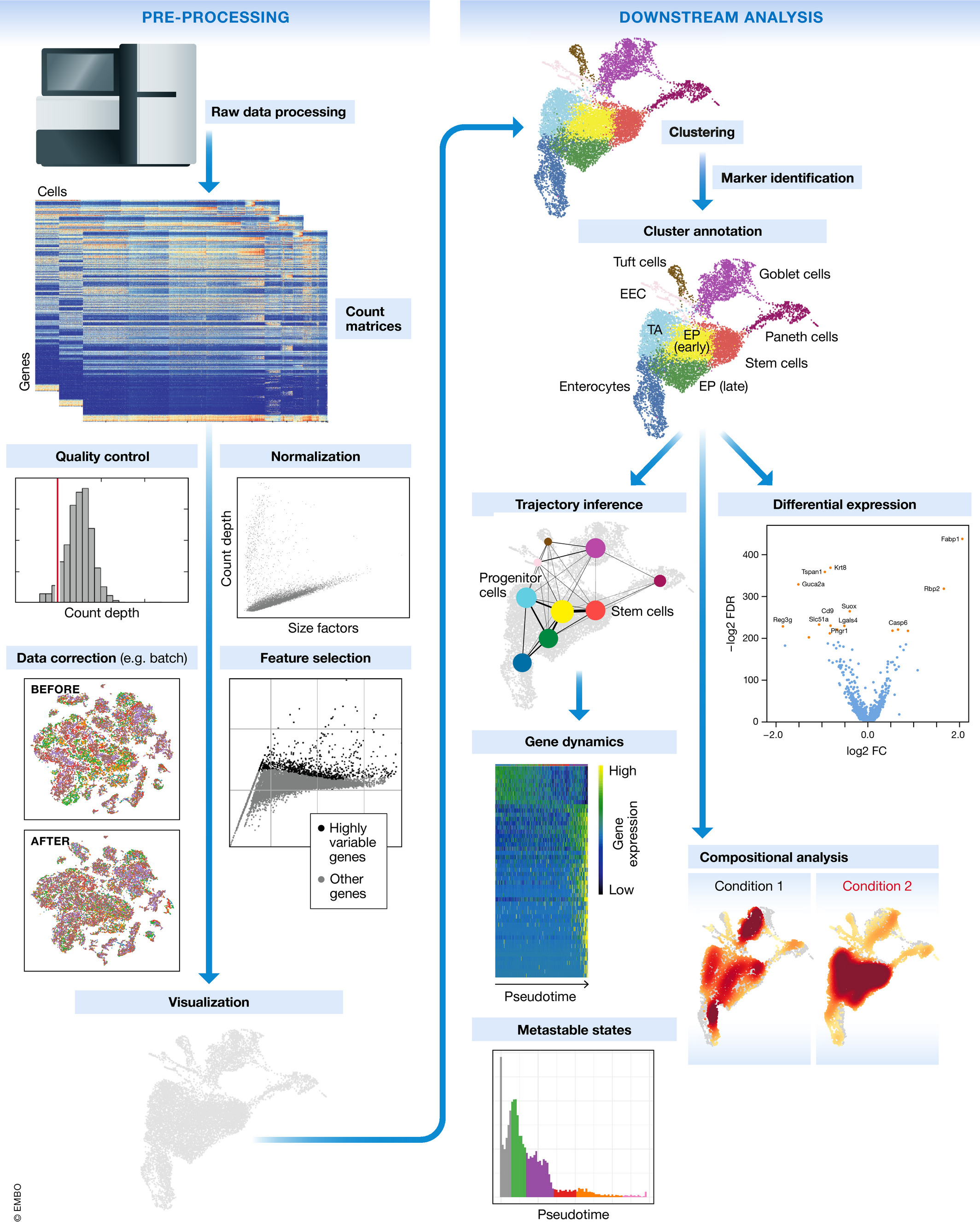
The general workflow that is followed in scrnaseq is shown in Figure 5.

Figure 5: General workflow of scRNA-seq. Image obtained from here.

Once you get the reads from sequencing facility, they will either be in BCL or FASTQ format or count matrix. Although most of the sequencing facilities nowadays would usually gives the sequencing file in FASTQ format. In case you are given the file in BCL format the first step would be to convert them to FASTQ format which can easily be done using Illumina bcl2fastq or for instance if one is using CellRanger pipeline then they have provide the useful function in the pipeline cellranger mkfastq which is preferred option for converting BCLs to FASTQs. However, if one wants to use the CellRanger pipeline then using their function cellranger mkfastq is the preferred one because it will generate cell-Ranger compatible FASTQs. More details on Cell-Ranger pipeline is here.

Quality Check:

After getting FASTQs, the first step generally that is common in almost all the high-throughput sequencing is running a quality control on FASTQ file and usually this is done utilizing FASTQC user guide page . Overall, FASTQC generate an html or this. Here:i am attaching a link to one of the very useful resources that can get you started with FASTQC ,how to interpret it and what is good and bad quality. This material was taken from this course:Bioinformatics for Biologists: Analysing and Interpreting Genomics Datasets that was offered by wellcome connecting science and is one of the best course if someone is interested in analyzing genomics dataset and variant interpretation. Nevertheless, FASTQC generates a QC report for each input FASTQ file, essentially summarizes the quality score, base content, and certain relevant statistics to spot potential problems originating from library preparation or sequencing. Additionally, another tools that can give more comprehensive report is MultiQC, the output file of which looks something like this.

Mapping:

1. Alignment or mapping refers to the process of matching the sequenced RNA reads to a reference genome or transcriptome. This step is crucial for identifying the origins of fragments especially RNA in the context of scRNA within each cell, enabling the quantification of gene or transcript expression levels. This step is usually computationally intensive in any high-throughput sequencing analysis.

2. The alignment process uses specialized algorithms to locate the positions of RNA reads on the reference genome, thus determining which genes are expressed and at what levels.

3. The output of this process typically includes several key files: an aligned reads file in BAM (Binary Alignment Map) or SAM (Sequence Alignment Map) format, which contains detailed information about the read sequences, their alignment positions, and mapping quality; a gene expression matrix in tabular format, which provides counts of reads or transcripts mapped to each gene for every single cell, essential for downstream analyses like identifying differentially expressed genes and clustering cells based on their gene expression profiles.

4. Summary statistics that assess the quality of the alignment, including metrics such as the percentage of successfully aligned reads, the distribution of reads across genomic features, and overall coverage depth. Through alignment or mapping, researchers can accurately quantify gene expression at the single-cell level, facilitating insights into cellular heterogeneity and the discovery of novel cell types and states.

5. As of now, several tools has been developed to align or map scRNA reads to either reference transcriptome, genome or an augmented transcriptome. Tools like Cell Ranger (Zheng et al. 2017), zUMIs (Parekh et al. 2018), alevin (Srivastava et al. 2016), Raindrop (Niebler et al. 2020), kallisto Bustools (Melsted et al. 2021), STARsolo (Kaminow, Yunusov, and Dobin 2021), and Allevin fry (He et al. 2022) are some of the tools that have been extensively used to carry out alignment or mapping.

Different reference sequences can be used for mapping. There are three main types of reference sequences:

• The full, annotated reference genome.

• The annotated transcriptome.

• Mapping against an augmented transcriptome.

However, it’s important to note that not all combinations of mapping algorithms and reference sequences are currently possible. For instance, there are no lightweight mapping algorithms available that can perform spliced mapping of reads against a reference genome.

Mapping using reference Genome:

• Mapping in scRNA-seq involves aligning sequenced RNA reads to the entire genome of the target organism, including annotated transcripts.

• Tools like zUMIs, Cell Ranger, and STARsolo use this whole-genome approach.

• These tools employ splice-aware alignment algorithms to handle reads from spliced transcripts, meaning they can align reads split across splicing junctions.

• The advantage of this method is that it accounts for reads from any location in the genome, not just known transcripts.

• This approach allows capturing reads within introns and other non-annotated regions, enabling comprehensive gene detection and quantification.

• Constructing a genome-wide index is required, which allows reporting reads that map to both known spliced transcripts and intronic regions.

• Such methods can also capture reads outside annotated transcripts, which helps in post hoc augmentation of quantified loci, increasing gene detection sensitivity.

• However, this method requires substantial memory, especially during the index construction and storage phase, often exceeding hundreds of gigabytes.

• Using a sparse suffix array can reduce the index size but at the cost of alignment speed.

• Spliced alignment is more computationally expensive than contiguous alignment due to the complexity of explicitly computing alignment scores for each read.

• This approach necessitates the availability of the organism’s genome, which can be challenging for non-model organisms that only have a transcriptome assembly available.

Mapping using Reference Transcriptome:

• To reduce the computational load of spliced alignment to a genome, an alternative approach is to use only the sequences of annotated transcripts as the reference.

• Most single-cell experiments use model organisms (like mice or humans) that have well-annotated transcriptomes, making transcriptome-based methods provide similar read coverage to genome-based methods.

• Transcriptome sequences are smaller than genome sequences, which reduces the computational resources needed for the mapping process.

• Using transcript sequences, which already include splicing patterns, eliminates the need for complex spliced alignment. Instead, reads are mapped through contiguous alignments.

• This approach works well with both alignment and lightweight mapping techniques, and is used in many popular tools.

• However, this method doesn’t capture reads from outside the spliced transcriptome, making it unsuitable for single-nucleus data.

• In single-cell experiments, reads from outside the spliced transcriptome can be significant and should be included in the analysis.

• Using lightweight mapping approaches can sometimes lead to incorrect read mappings and unrealistic estimates of gene expression.

Mapping against an augmented transcriptome:

An augmented transcriptome is an updated version of a standard transcriptome reference that includes additional sequences beyond the typical spliced transcripts. This augmentation can involve the inclusion of:

• Full-Length Unspliced Transcripts: These are the complete RNA sequences before splicing occurs, which include both exons and introns.

• Intronic Sequences: These are the sequences of introns, which are usually removed during the splicing process in eukaryotic cells.

• Other Non-Coding Regions: Additional sequences that may give rise to RNA reads, such as untranslated regions (UTRs) or intergenic regions.

• To account for reads that may come from outside of spliced transcripts, spliced transcript sequences can be augmented with additional reference sequences, such as full-length unspliced transcripts or intronic sequences.

• Augmented transcriptome references, which include introns, create reference indices that are smaller than those needed for the full genome while still enabling the search for contiguous read alignments.

• This approach can lead to faster and less memory-intensive alignment compared to mapping against the full genome, while also capturing many reads from outside the spliced transcriptome.

• Mapping to an expanded set of reference sequences recovers more reads than mapping to the spliced transcriptome alone, and reduces spurious mappings when using lightweight mapping-based methods.

• Augmented transcriptomes are useful for quantifying single-nucleus data or preparing data for RNA-velocity analysis, offering a balance between computational efficiency and comprehensive read mapping.

• (He et al. 2022) recommend constructing an augmented splici (spliced + intronic) reference even for standard single-cell RNA-seq data. This reference combines spliced transcript sequences with intronic sequences of annotated genes. Using this splici reference allows lightweight mapping methods, reduces spurious mappings, and improves sensitivity by detecting both spliced and unspliced reads.

• During quantification, splicing status is tracked and reported separately, unifying the preprocessing pipeline for single-cell, single-nucleus, and RNA-velocity analysis.

Considerations Regarding Mapping:

Here I am attaching a shell file: prepare_reference.sh that contains all the script on downloading reference genome and annotation file and then some minor changes to make it more cellRanger-compatible. Additionally if you are working on mouse data then go to this link and you will find all the relevant information regarding mouse data. When mapping reads to transcriptome one needs to consider:

1. If a Knock-in mouse has a novel human gene inserted into its genome, it is necessary to add that gene to the reference genome to accurately quantify its expression.

2. Annotation quality needs to be considered, especially when working with non-model species. For mouse or human, this is generally not an issue. However, with non-model species, incomplete or inaccurate annotations can cause problems, particularly when sequencing only one end of the transcript. If many transcripts have long untranslated regions (UTRs) that have not been identified, it could result in the loss of a significant number of reads and genes. This is because many reads might not map to the annotated gene body. Therefore, it may be necessary to update the annotation if working with a less well-characterized genome of a non-typical species.

3. Consider whether to include introns and exons or just exons. Previously, the answer was to use exons only for single-cell RNA sequencing and both introns and exons for single-nucleus RNA sequencing. However, now Cell Ranger includes both by default, as it captures 20% more reads even for single-cell RNA sequencing. There are also methods that utilize intronic versus exonic information, such as scVelo,(Soneson et al. 2021) which requires separate quantification of intron and exon reads.

   For assigning reads to cells, the correct whitelist for cell barcodes is needed, and UMIs (unique molecular identifiers) are counted. One challenge is dealing with multi-mapping reads, where a read maps to multiple genes so which gene gets UMI count for that read. Cell Ranger’s current rule is to exclude all those reads that are multimapping, which can lead to an undercounting bias for genes with close homologs.

   Cell Ranger also addresses sequencing errors in UMIs by allowing for up to one base pair error in the UMI sequence and correcting for it. While Cell Ranger is commonly used for 10x Genomics data, there are alternatives like STARsolo, which mimics Cell Ranger but is open-source and allows for easier modification of parameters.

4. I’ve been discussing sequencing errors, which might seem unusual to those familiar with sequencing technology, as it is typically 99.9% accurate these days. However, when I mention sequencing errors, I’m actually referring to all the errors that can occur from the mRNA molecules to our sequencing reads. Errors can arise from reverse transcriptase during cDNA synthesis, from DNA polymerase during sequence amplification, and from the sequencing machine itself. While the sequencing machine’s errors are very low, errors at other stages are not necessarily as minimal.

What other things that could possibly go wrong😧:

Before explaining what other things could possibly go wrong, its time to define few terminologies.

Ambient RNA: Ambient RNA is cell-free mRNA that is released during preparation of single-cell suspensions for scRNA-Seq analysis.

Doublets: A doublet in scRNA-seq refers to an event where two cells are captured in the same droplet or well, leading to their RNA being sequenced together.

Lets explore the ambient RNA thing in detail now, but first we need to know how the droplets are generated.

How are droplets generated in an ideal world:

To explain the process of empty droplet generation in single-cell assays, we need to look at how these droplets are created. We produce these droplets by simultaneously flowing barcoded beads and cells, which are then encased in droplets by oil in our 10x Chromium machine as shown in Figure 6.

Figure 6: How droplets are generated

This process generates hundreds of droplets per second. Ideally, each droplet would contain one cell and one barcoded bead, but in reality, only about 5% of the droplets achieve this ideal condition. Additionally, all droplets contain ambient RNA. This occurs because some cells get damaged or break during handling and extraction from tissue, particularly when passing through microfluidic devices at high speeds. This results in RNA being released into the surrounding solution.

When droplets are formed, they capture both the cells and the ambient RNA floating in the supernatant. Therefore, ambient RNA is present in nearly all droplets. In practice, about 95% of droplets are considered empty, with approximately 20% containing only ambient RNA. Around 7% of droplets will have a barcoded bead with capture nucleotides along with ambient RNA as shown in Figure 7.

Figure 7: Possible droplets Configuration

This means the barcoded bead can capture ambient RNA, generate cDNA, and include unique molecular identifiers (UMIs) that will appear in the sequencing library and subsequently in the sequencing data results.

When ambient RNA is present at moderate to high levels, it can cause problems in later parts of the analyses for two main reasons:

1. Ambient RNA can mix with the genuine gene expression profiles of cells, making it difficult to accurately identify cell types.

2. Differences observed between experimental conditions might be due to variations in ambient RNA levels rather than actual biological differences.

3. For the solution of this problem (Lun et al. 2019) proposed an efficient method in this paper and that cell Ranger Version 3 and above has adapted in their pipeline. For the detail method here is the link to the paper (Lun et al. 2019). The function emptydrops is embedded in DropletUtils R package. Another useful resource for When should I correct for ambient RNA?

2nd Problem: Processed pseudogenes are mRNAs that have undergone reverse transcription within the cell and been reintegrated into the genome. They possess the entire exonic sequence but lack promoters, enhancers, or any regulatory elements, making them incapable of being expressed since transcription factors or RNA polymerase cannot bind to them.

Despite this, we still detect them due to mismatched reads. Ideally, all reads should align with the gene that is actively transcribed, but a small portion of reads actually map to the processed pseudogene. This mismapping accounts for about 4% of the reads. Considering a 1% sequencing error rate, a 100 base pair read would result in approximately 4% of the reads having three or more sequencing errors, causing mismapping. This analysis only includes uniquely mapping genes, excluding multimapping reads.

To address this mismapping issue, the default genome provided by cellRanger masks all pseudogenes and processed pseudogenes. This masking is done to prevent errors caused by mismatched reads.

Doublet Problem:

• Doublets in single-cell RNA sequencing (scRNA-seq) arise when two cells are captured together in the same droplet or well during the encapsulation process as shown in Figure 7. Multiple cells with multiple beads but that is less common.

• Doublets are divided further into two categories:

• Heterotypic Doublets: When one bead capture two different cells where one could be an epithelial cell and one could be a T-cell.

• Homotypic Doublets: When one bead capture two same cells, where both the cell are of the same type such as T-cells.

• Sadly, at this stage we cannot do anything about homotypic doublet and this is an active area of research. Andrews Computation Biology Lab is working actively on this side of the single cell and ambient RNA as well. Anyone interested in this can go and check out their lab.

• But their are a bunch of tools that have been developed which works efficiently on identifying these heterotypic doublets i.e Doublet finder, Scrublet.

Be ashamed to die until you have won some victory for humanity: Horace Mann

References

Aird, Daniel, Michael G Ross, Wei-Sheng Chen, Maxwell Danielsson, Timothy Fennell, Carsten Russ, David B Jaffe, Chad Nusbaum, and Andreas Gnirke. 2011. “Analyzing and Minimizing PCR Amplification Bias in Illumina Sequencing Libraries.” Genome Biology 12 (2): R18. https://doi.org/10.1186/gb-2011-12-2-r18.

Archer, Nathan, Mark D Walsh, Vahid Shahrezaei, and Daniel Hebenstreit. 2016. “Modeling Enzyme Processivity Reveals That RNA-Seq Libraries Are Biased in Characteristic and Correctable Ways.” Cell Systems 3 (5): 467–79.

He, Dongze, Mohsen Zakeri, Hirak Sarkar, Charlotte Soneson, Avi Srivastava, and Rob Patro. 2022. “Alevin-Fry Unlocks Rapid, Accurate and Memory-Frugal Quantification of Single-Cell RNA-Seq Data.” Nature Methods 19 (3): 316–22. https://doi.org/10.1038/s41592-022-01408-3.

Kaminow, Benjamin, Dinar Yunusov, and Alexander Dobin. 2021. “STARsolo: Accurate, Fast and Versatile Mapping/Quantification of Single-Cell and Single-Nucleus RNA-Seq Data.” http://dx.doi.org/10.1101/2021.05.05.442755.

Lun, Aaron T. L., Samantha Riesenfeld, Tallulah Andrews, The Phuong Dao, Tomas Gomes, and John C. Marioni. 2019. “EmptyDrops: Distinguishing Cells from Empty Droplets in Droplet-Based Single-Cell RNA Sequencing Data.” Genome Biology 20 (1). https://doi.org/10.1186/s13059-019-1662-y.

Melsted, Páll, A. Sina Booeshaghi, Lauren Liu, Fan Gao, Lambda Lu, Kyung Hoi Min, Eduardo da Veiga Beltrame, Kristján Eldjárn Hjörleifsson, Jase Gehring, and Lior Pachter. 2021. “Modular, Efficient and Constant-Memory Single-Cell RNA-Seq Preprocessing.” Nature Biotechnology 39 (7): 813–18. https://doi.org/10.1038/s41587-021-00870-2.

Niebler, Stefan, André Müller, Thomas Hankeln, and Bertil Schmidt. 2020. “RainDrop: Rapid Activation Matrix Computation for Droplet-Based Single-Cell RNA-Seq Reads.” BMC Bioinformatics 21 (1). https://doi.org/10.1186/s12859-020-03593-4.

Parekh, Swati, Christoph Ziegenhain, Beate Vieth, Wolfgang Enard, and Ines Hellmann. 2018. “zUMIs - A Fast and Flexible Pipeline to Process RNA Sequencing Data with UMIs.” GigaScience 7 (6). https://doi.org/10.1093/gigascience/giy059.

Soneson, Charlotte, Avi Srivastava, Rob Patro, and Michael B. Stadler. 2021. “Preprocessing Choices Affect RNA Velocity Results for Droplet scRNA-Seq Data.” Edited by Min Li. PLOS Computational Biology 17 (1): e1008585. https://doi.org/10.1371/journal.pcbi.1008585.

Srivastava, Avi, Hirak Sarkar, Nitish Gupta, and Rob Patro. 2016. “RapMap: A Rapid, Sensitive and Accurate Tool for Mapping RNA-Seq Reads to Transcriptomes.” Bioinformatics 32 (12): i192–200. https://doi.org/10.1093/bioinformatics/btw277.

Zheng, Grace X. Y., Jessica M. Terry, Phillip Belgrader, Paul Ryvkin, Zachary W. Bent, Ryan Wilson, Solongo B. Ziraldo, et al. 2017. “Massively Parallel Digital Transcriptional Profiling of Single Cells.” Nature Communications 8 (1). https://doi.org/10.1038/ncomms14049.